On Verification

Those who are new to scientific computing often underestimate the importance of verification and validation (V&V). Verification is the process of ensuring that your code solves the governing equations correctly, whereas validation involves demonstrating that your model accurately simulates reality by comparing to empirical data. V&V is the cornerstone of computational modeling and should be done every time you create a computational model. The process should be done carefully and methodically, building confidence in your model.

In this post, I will discuss the process of verification and will show how I use verification to build confidence in a model I created. The model I use in the example that follows computes the trajectory of a 2D object undergoing projectile motion and coming in contact with a flat surface. The model is a simpler version of a 3D model I am creating to simulate the trajectory of firebrands (i.e., embers from a wildfire) coming in contact with a roof.

Formulation

Before we can talk about verification, we need a computational model. Consider a 2D object with initial position $(x_0, y_0)$ and velocity $(v_{x0}, v_{y0})$ . When the object is in the air, it is subjected to the forces of gravity $F_g = mg$ and drag $F_d = \frac{1}{2} \rho AC_d v^2$ , as shown in the figure. Here, m is mass, g is gravitational acceleration, $\rho$ is the density of air, A is the area perpendicular to the motion, $C_d$ is the drag coefficient, and v is velocity.

The equations of motion are

$m \frac{dv_x}{dt}=F_x$

$m \frac{dv_y}{dt}=F_y$

where $F_x$ and $F_y$ are the x and y components of the resultant force acting on the object. Additionally,

$\frac{dx}{dt}=v_x$

$\frac{dy}{dt}=v_y$

When the object comes in contact with a flat surface oriented at angle $\alpha$ with respect to the global x axis, we define two behaviors: bouncing and sliding. In reality, the object may roll as well, but we will ignore that behavior for the time-being.

For bouncing, we define e as the coefficient of restitution, which is a number between 0 and 1 that accounts for the degree of inelasticity in the collision (i.e., e=1 means a perfectly elastic collision and e=0 means a perfectly inelastic collision). The velocities before (“1”) and after (“2”) impact are transformed into their normal n and tangential t components. From vector algebra,

$v_{t1} = v_x \cos \alpha + v_y \sin \alpha$

$v_{n1} = v_y \cos \alpha - v_x \sin \alpha$

The velocities before and after impact are shown in the figure below.

Normal and tangential velocities before (“1”) and after (“2”) impact

Then,

$v_{t2}=v_{t1}$

$v_{n2}=-ev_{n1}$

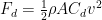
Note that friction forces are also present when the object is in contact with the surface. As shown in the figure below, the friction force is $F_f=\mu mg \cos \alpha$ , where $\mu$ is the coefficient of kinetic friction. The friction force is included in the net force acting on the object during times that the object is in contact with the surface.

Free-body diagram for object in contact with surface showing friction force

Numerical Model

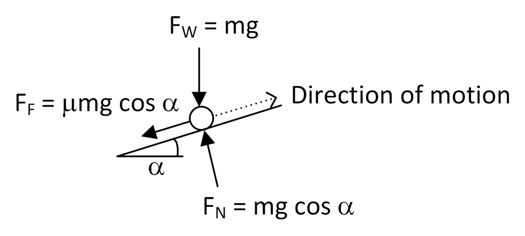
The equations of motion are solved numerically using the fourth-order Runge-Kutta method [1]. In the Runge Kutta method, the function is projected forward with a slope that depends on the order of the analysis. For this type of analysis, the time step $\Delta t$ must be specified. By using an approximate slope and discretizing time in this manner, the analysis is no longer exact, although errors can be managed.

The equations of motion are dependent on whether the object is in contact with the surface or not. It is assumed that the object is in free fall until contact is detected (which is based on whether its computed coordinates pass the surface’s boundary within a specified tolerance $\epsilon$ . Mathematically, contact occurs when

$-\epsilon < y-x \tan \alpha < \epsilon$

Since it is possible that the computed coordinates overshoot the boundary, the bisection method [1] is used to determine a precise time when the object is within to tolerance.

Defining contact with surface at angle $\alpha$

Defining contact with surface at angle $\alpha$

Once contact has been identified, the normal and tangential velocity equations that define friction and sliding behaviors are invoked. To provide some stability to the solution, the velocity is set to zero when its magnitude is less than the tolerance, and once the velocity is zero, it remains zero.

The details of the calculations are left out for brevity. The computational model was implemented in Python, and the code was systematically debugged using the verification cases shown below.

Verification Process

Verification is an iterative process, and the problems chosen for verification should be analyzed anytime a change in the code is made. Because you are verifying that your code is solving the equations correctly, you should be able to test the convergence properties of your model.

Two types of verification problems exist. In the first case, an analytical solution is available, meaning that you are comparing your model to an “exact” answer. In the second case, you may have a problem that is too complex to solve analytically. Here, you might seek to compare your model to an existing model. Note that you can no longer show that your answer converges to the true solution. However, you can have some level of confidence if you can arrive at the same answer as someone else.

In assessing the accuracy of your solution, it is necessary to express your solution in terms of a percent error, either the true error (when an analytical solution exists) or an approximate error (when comparing to another model). The formula for calculating error is

$\texttt{error} = \frac{\texttt{computed value}-\texttt{known value}}{\texttt{known value}} \times 100 \%$

When selecting verification cases, you should select problems that isolate the various levels of complexity in your model. For the model shown here, we have the following:

Projectile motion without/with air resistance: Does the object reach the ground at the correct time and location? Does the trajectory match the theoretical solution?
Bouncing: Does the distance traveled and the time for the object to come to a stop match the theoretical solution?
Sliding with friction: For an object on an incline, does the distance traveled and the time for the object to come to a stop match the theoretical solution?

For each of these cases, it is important to demonstrate the convergence behavior of the model. Namely, as you successively cut the time step in half, the error should systematically reduce according to the order of the model. The order can be observed on a log-log plot of time step versus the absolute value of the error for varying time steps. I don’t show this in the example that follows but there are plenty of examples on the web.

Verification of the Current Model

Projectile Motion without Air Resistance

Consider a spherical object with mass m = 145 g and radius r = 3.75 cm with initial velocity of 30 m/s launched from the ground at an angle of $45^\circ$ . Ignoring drag, the time and distance traveled until the object hits the ground is

$t^* = \frac{v_{0,y}}{0.5gt} = 4.3248$ s

$x^* = v_{0,x} t^* = 91.743$ m

This solution can be found in most physics textbooks.

Using the code, the ball is expected to first hit the ground at $t^* =4.3248$ s with a distance traveled of $x^* = 91.743$ m. The error is negligible (i.e., less than the tolerance). Note that time step has little influence on the accuracy of the simulation up to the first impact. The figure below shows the trajectory for time steps ranging from 0.1 s to 0.0001 s, and there is virtually no difference in the computed solution. Furthermore, due to the use of the bisection algorithm, time step has no influence on the accuracy of $t^*$ and $x^*$ .

Projectile Motion with Air Resistance

The drag force changes the trajectory of an object and reduces the distance traveled and time to impact. Chudinov [2] derived analytical expressions for several parameters that define the trajectory of objects in projectile motion with air resistance, namely, the peak ascent of the object H, the time to impact $t^*$ , and the flight range $x^*$ , among others. Specifically,

$H= \frac{v_0^2 \sin ^2 \theta_0}{g(2+kv_0^2 \sin \theta_0)}$

$t^*=2 \sqrt{\frac{2H}{g}}$

$x^*=v_at^*$

where $k = \frac{\rho C_d A}{2mg}$ is a constant and the velocity at the apex $v_a$ is given by

$v_a= \frac{v_0 \cos \theta_0}{\sqrt{1+kv_0^2(\sin \theta_0 + \cos ^2 \theta_0 \ln \tan (\frac{\theta_0}{2}+\frac{\pi}{4}}))}$

Consider again a spherical object with mass m = 145 g and radius r = 3.75 cm with initial velocity of 30 m/s launched from the ground at an angle of $45^\circ$ . $\rho = 1.225$ kg/m $^3$ and $C_d = 0.5$ .

The table below shows the time at impact and the horizontal distance traveled in comparison to the analytical solution. You can see that errors are within 1 percent. Moreover, refining the time step does not improve the solution due to the process used in the bisection algorithm.

Bouncing

According to Nagurka [3], a ball with zero initial velocity dropped on a flat surface from height $y_0$ with coefficient of restitution e will theoretically bounce until

$t = \frac{1+e}{1-e} \sqrt{\frac{2y_0}{g}}$

The total distance traveled along the path s is

$s = [ 1+2 \sum_{i=1}^{\infty} e^{2i} ] y_0$

In the equations provided by Nagurka, drag and friction forces are neglected.

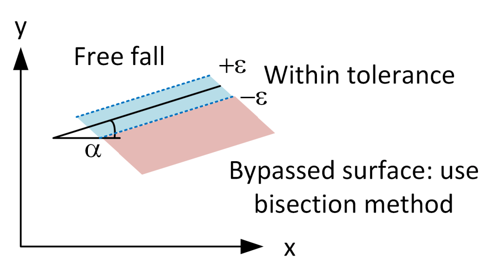
Consider now an object with $y_0 = 1$ m and e = 0.8. According to theory, the particle will stop bouncing at t = 4.064 s. The vertical distance traveled is s = 4.556 m.

The figure below shows the computed height of the particle as a function of time for various time steps. Good agreement is achieved for most of the analysis. Deviations occur as time progresses, with bounces becoming more out of sync as the particle approaches a stationary configuration.

Bouncing with e = 0.8 for various time steps

The following table shows the computed time until the particle stops bouncing as well as the total distance traveled along the path. You can see that the computational model gives good agreement, with errors less than one percent for $\Delta t = 0.0001$ s.

Sliding with Friction

To verify the friction force calculation, consider a block on an incline at angle $\alpha$ with initial velocity $v_0$ and a coefficient of kinetic friction $\mu$ . You can look in most textbooks and find that the block moves with acceleration

$a = g \sin \alpha + \mu g \cos \alpha$

The distance s traveled before the block comes to rest is

$s = -\frac{v_0^2}{2a}$

The time until the block comes to rest is

$t = -\frac{v_0}{a}$

The distance traveled and the time to reach zero velocity for angles $\pm 15 ^\circ$ were analyzed using the code. The table below shows the result for $\alpha = +15 ^\circ$ , in which the initial velocity was 10 m/s up the slope. The coefficient of kinetic friction is $\mu = 0.75$ . Similar levels of accuracy were obtained for $\alpha = -15 ^\circ$ , with the initial velocity of 10 m/s down the slope. You can see that a time step of 0.01 s gives results within 1 percent accuracy.

Conclusions

Through the process of verification, I was able to find and correct bugs in my code. I am confident now that the code is accurate for simulating the 2D problem I set out to model. When you do verification, I recommend that you systematically refine your mesh and time step and calculate errors. This will show you that your model is converging to the true solution. As you move forward, you may wonder, what is the best time step or mesh density for my model? Honestly, it is ultimately up to you, the modeler. You need to balance accuracy with computational efficiency. In the simple model shown here, the simulation times were negligible, but if I attempt to model a larger or more complex problem, then I will need to think about the computational resources needed to run a simulation. That’s a topic for a different time 🙂

References

[1] Chapra, S.C., and Canale, R.P. (2010). Numerical Methods for Engineers, McGraw Hill: New York, NY.

[2] Chudinov, P.S. (2004). “Analytical investigation of point mass motion in midair,” European Journal of Physics, 25, 73-79.

[3] Nagurka, M. (2003) “Aerodynamic effects in a dropped ping-pong ball experiment,” International Journal of Engineering Education, 19, 623-630.

	$t^*$	Error (%)	$x^*$	Error (%)
$\Delta t = 0.1$	3.7533	-0.9488	57.167	0.1377
$\Delta t = 0.01$	3.7533	-0.9488	57.167	0.1377
Analytical	3.7892		57.088

	t (s)	Error (%)	s (m)	Error (%)
$\Delta t = 0.01$	3.032	-25.40	4.185	-8.126
$\Delta t = 0.001$	3.829	-5.770	4.478	-1.691
$\Delta t = 0.0001$	4.040	-0.5939	4.539	-0.1129
Exact	4.064		4.556

	t (s)	Error (%)	s (m)	Error (%)
$\Delta t = 0.1$	1.100	6.106	5.177	-0.1254
$\Delta t = 0.01$	1.040	0.3202	5.183	-0.004166
Exact	1.037		5.184

A. E. Jeffers

Ann E. Jeffers, Ph.D.

On Verification

Formulation

Numerical Model

Verification Process