I’m a big fan of coding, but I get the sense my college education may have failed me. Don’t get me wrong–I’m proud of my degrees from Pitt and Virginia Tech, and my education was more than enough to propel me into an academic career at the University of Michigan. But the state of the art for computer analysis in civil engineering in the early 2000s was the brute force structure of procedural languages like FORTRAN. Object-oriented programming (OOP) was a topic left to the computer scientists.

Twenty years later, I still follow the old habits that were drilled into my head as an undergrad. However, I’ve been working more and more in modern languages like Python due to courses I teach on computational analysis. Python is an open source language with countless libraries that can be downloaded seamlessly. It is a powerful tool that can do so much more than the languages from the days of yore. Python’s capacity for OOP has always intrigued me, but I wasn’t prompted to teach myself OOP until my eleven year old asked me to help program a video game (more on that later).

I’m sharing what I learned so other engineers (especially older folks like me) are encouraged to realize the power behind OOP. To follow along, you need Python 3. ​I recommend downloading Anaconda for scientific computing in general, and Jupyter Notebook is the quickest way to get started with coding in Python.

Defining Classes

In OOP, the properties and functions attributed to an instance are based on classes. Classes are defined in Python according to the following convention:

class ClassName:
    def __init__(self, x1, x2, ..., xN):
        self.data = self
        self.x1 = x1
        self.x2 = x2
        ...
        self.xN = xN

The first line defines a class with the name “ClassName.” Note that the first letter of the class name is capitalized per convention. The function __init__(self, x1, x2, …, xN) initializes an instance of the class with properties x1, x2, …, xN. Every instance is characterized by its name (“self”) and its properties. 

Suppose we want to create a class TrussElements to do linear analysis of trusses. The properties that we associate with a truss element are the x and y coordinates of its two nodes, the cross-sectional area, and Young’s modulus. The class definition would be as follows:

class TrussElements:
    def __init__(self, x1, y1, x2, y2, area, E):
        self.data = self
        self.x1 = x1
        self.y1 = y1
        self.x2 = x2
        self.y2 = y2
        self.area = area
        self.E = E

Creating Instances of Objects

Once the class is defined, we then create instances of truss elements by calling on the class.  Consider the truss in the figure below. Member AB has an area of 2.5 in.^2 and member BC has an area of 1 in.^2. Both members have Young’s modulus of 30,000 ksi. A force of 5 k is applied at joint B, and we might be interested in calculating the displacements at the nodes, the reaction forces at the supports, and the axial force in each member of the truss (we won’t do all that here, but we will set the problem up). 

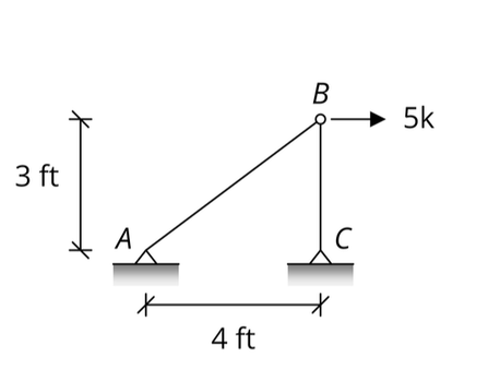
We create instances of truss elements by calling on TrussElements with the appropriate values for x1, y1, x2, y2, area, and E. Note that we do not need to pass “self” into the class because it is implied by the name we give the instance. For our two bars, AB and BC, we have:

AB=TrussElements(0, 0, 48, 36, 2.5, 30000)
BC=TrussElements(48, 36, 48, 0, 1, 30000)

Now that we have created the instances, we can call on their properties. For example, if we want to print the area of element AB, we can do that. If we want to print Young’s modulus of element BC, we would do the following:

print(AB.area)
print(BC.E)

This returns the values 2.5 and 30000. You can see that it is now convenient for us to call on the instance and its properties using the “.” notation.

Method Objects

In addition to ascribing attributes to classes, we can also ascribe methods (or functions) to classes. In the example of the truss, we may want to define a function to compute the length of the truss based on the coordinates of the end nodes. In the class definition, we will add a function Length that does this.  Note that we need to import the math library in this case to use the square root function. 

import math
class TrussElements:
    def __init__(self, x1, y1, x2, y2, area, E):
        self.data = self
        self.x1 = x1
        self.y1 = y1
        self.x2 = x2
        self.y2 = y2
        self.area = area
        self.E = E
    def Length(self):
        L = math.sqrt((self.x2-self.x1)**2+...
            (self.y2-self.y1)**2)
        return L

Now, calling on the Length function under each instance reports the length of the element:

print(AB.Length())
print(BC.Length())

Here we see the length of AB to be 60.0 and the length of BC to be 36.0. Note that the Length function does not have any arguments because the nodal coordinates are already a part of the class definition. 

Adding Output Statements to the Class

So far, we have used print statements outside of the class definition to print output. It may be convenient to format output to be the same for all instances of a class. This can be done using functions, but one particular function that may be of interest is the __str__() function, which modifies what appears when you print(Instance). 

​Consider our TrussElements class. We add the __str__() function to print as follows:

class TrussElements:
    def __init__(self, x1, y1, x2, y2, area, E):
        self.data = self
        self.x1 = x1
        self.y1 = y1
        self.x2 = x2
        self.y2 = y2
        self.area = area
        self.E = E
    def __str__(self):
        return f"Element goes from ({self.x1},...
            {self.y1}) to ({self.x2},{self.y2}). ...
             It has A = {self.area} and E = {self.E}"

Now when we print the instance, e.g., BC,

print(BC)

We obtain the following output: “Element goes from (48,36) to (48,0). It has A = 1 and E = 30000”.

Arrays of Classes

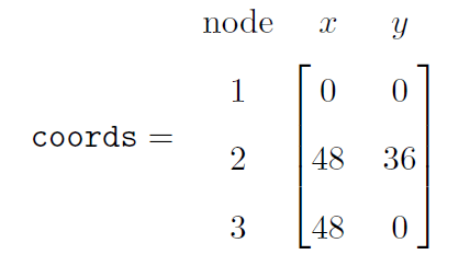
One final trick is that we can create arrays of classes. In the analysis of trusses, for example, we often loop over the elements in the structure and use an index to indicate the element under consideration. From the previous example, suppose we number AB as element 1 and BC as element 2. Joint A is node 1, joint B is node 2, and joint C is node 3. We will store coordinate information in a “coords” array. 

To use arrays, we must call upon the numpy library.

import numpy as np

Since we will loop over all elements (nels = 2), it is also convenient to store the areas in an array. We can also use a “connectivity” array to store the inode and jnode for each element. The connectivity array is as follows:

In Python, the input looks as follows:

nels = 2 
coords = np.array([[0,0],[48,36],[48,0]])
connectivity = np.array([[1,2],[3,2]])
area = np.array([2.5,1])
E = 30000

We initialize the truss array and enter a loop over the elements. For each element, we extract the nodal coordinates, area, and Young’s modulus, and enter them into the TrussElement class definition. We append the information for element i to the truss array. 

truss = []
for i in range(0,nels):
    inode = connectivity[i,0]
    jnode = connectivity[i,1]
    x1 = coords[inode-1,0]
    y1 = coords[inode-1,1]
    x2 = coords[jnode-1,0]
    y2 = coords[jnode-1,1]
    A = area[i]
    truss.append(TrussElements(x1,y1,x2,y2,A,E))

We can then print whatever output we need. For example,  the following prints the length, area, and E for each element. 

Summary

In this blog, we studied basic concepts of classes, instances, methods, and arrays as they apply to OOP. We looked at how these concepts can be applied to structural analysis by considering how data is stored for computational analysis of trusses. We have just scratched the surface of OOP, but hopefully you are inspired to learn more.